How To Flip Or Reverse Data In Microsoft Excel

Do you want to flip or reverse data in Microsoft Excel and are unsure on how to go about it?

This article will guide you on how to flip or reverse data in Microsoft Excel.

Unfortunately, MS Excel does not have an inbuilt option on this, but there are ways to do this. There is the MS Excel Sort feature that can be used to flip the data arranged alphabetically or numerically (smallest to largest or vice versa). The solutions provided in this article will be covering flipping or reversing unsorted and sorted data (alphabetically or numerically) vertically and horizontally.

How to fix the Excel Formula not updating Automatically?

The four options we will look into are:

1. How to switch or exchange rows and columns
2. How to flip or reverse a column
   • Using SORT and Helper column
   • Using a formula
3. How to flip or reverse a row (using SORT and Helper row)

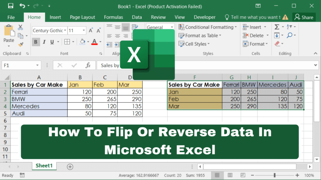
1. How to switch or exchange rows and columns

As much as a manual conversion of data on MS Excel from rows into columns or vice versa would be the viable option for most of us. However, when the size of the data is huge, this could end up being time-consuming. We will rotate the data below so that the data in the columns will be rearranged in rows.

Steps to follow:

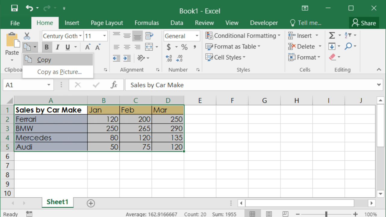
1. Select the data first that you would like to rearrange including the column and row labels or headers. Click on Copy under the Home tab or use shortcut keys CTRL+C

Tip: Ensure you use the copy command and not Cut command or CTRL+X

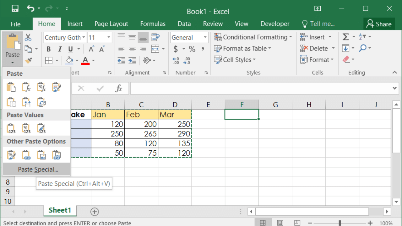
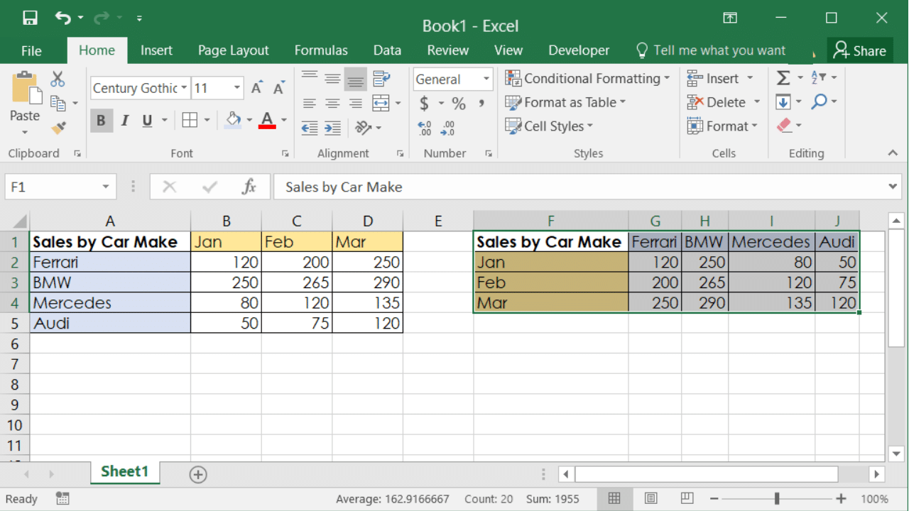
2. Select the cell you would like to paste the data to (in this case it is cell F1). Click on Home and click on the Paste icon drop-down arrow and select Paste Special.

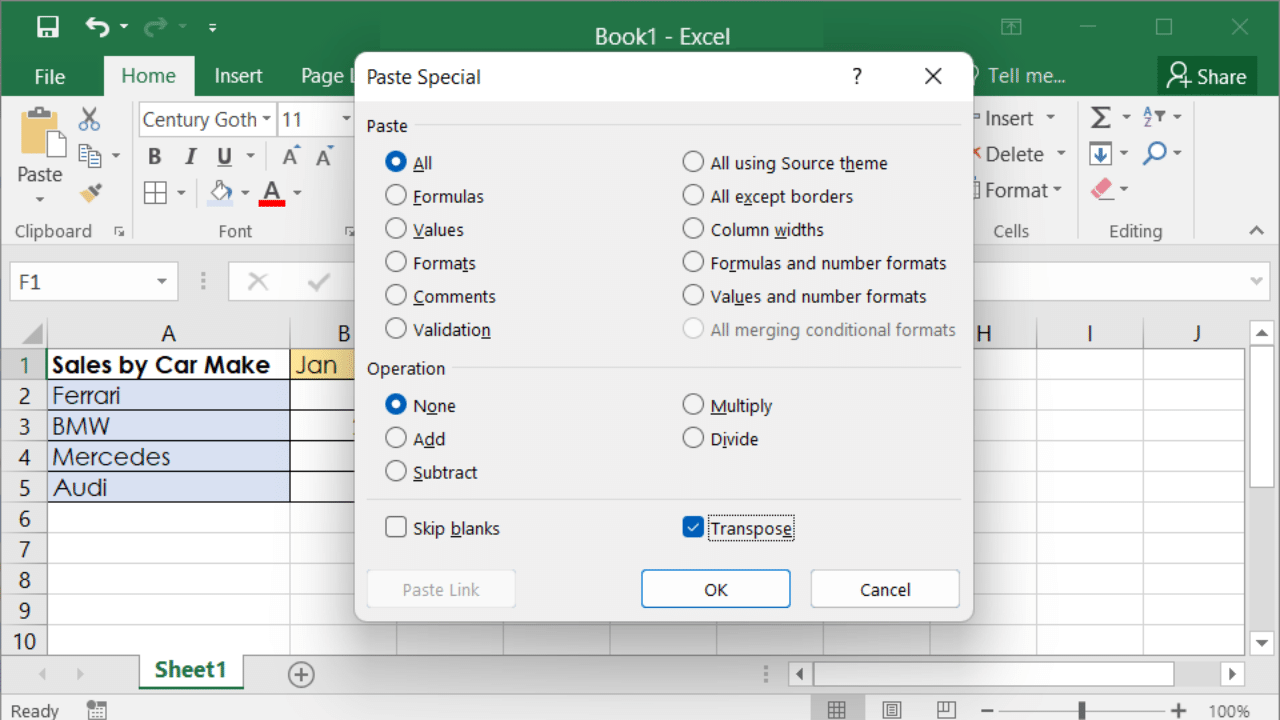
3. Select Transpose under Operation. Click on OK.

4. As a result of the completion of the above steps, the data in the columns will be rearranged in rows as per the image shown below.

2. How to flip or reverse a column

Below are 2 ways to flip a column:

2.1 Using SORT and Helper column

Microsoft Excel has a Sort Feature that you can use to easily reverse data in a column from bottom to top. This method of flipping requires an additional column Helper and the Sort Feature is then applied using the Helper column.

Steps to follow:

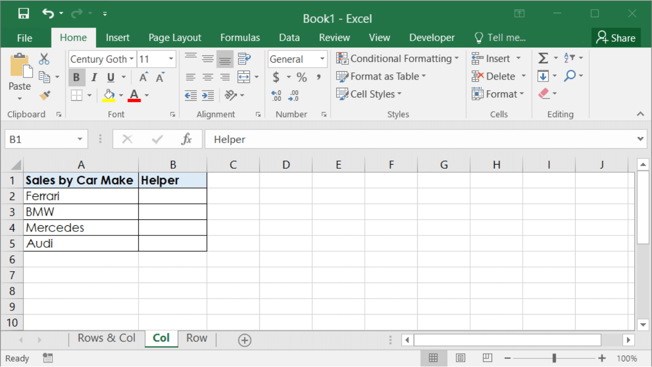
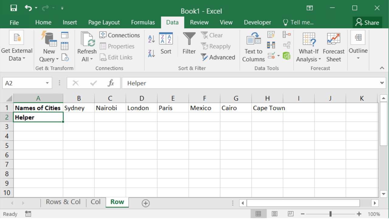
1. Enter Helper as the heading for a blank adjacent column.

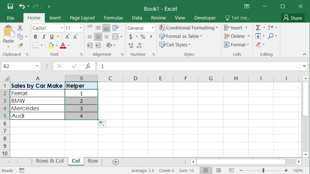
2. Enter a series of numbers start by entering 1 in the first cell, 2 in the second cell and then using the Fill handle (tip below) populate the Helper column up until the last item of the list.

Tip: Quick and easy way to number rows in MS Excel shown here to significantly save time.

3. Select all columns with data (columns A and B in this case) and go to the Data tab.

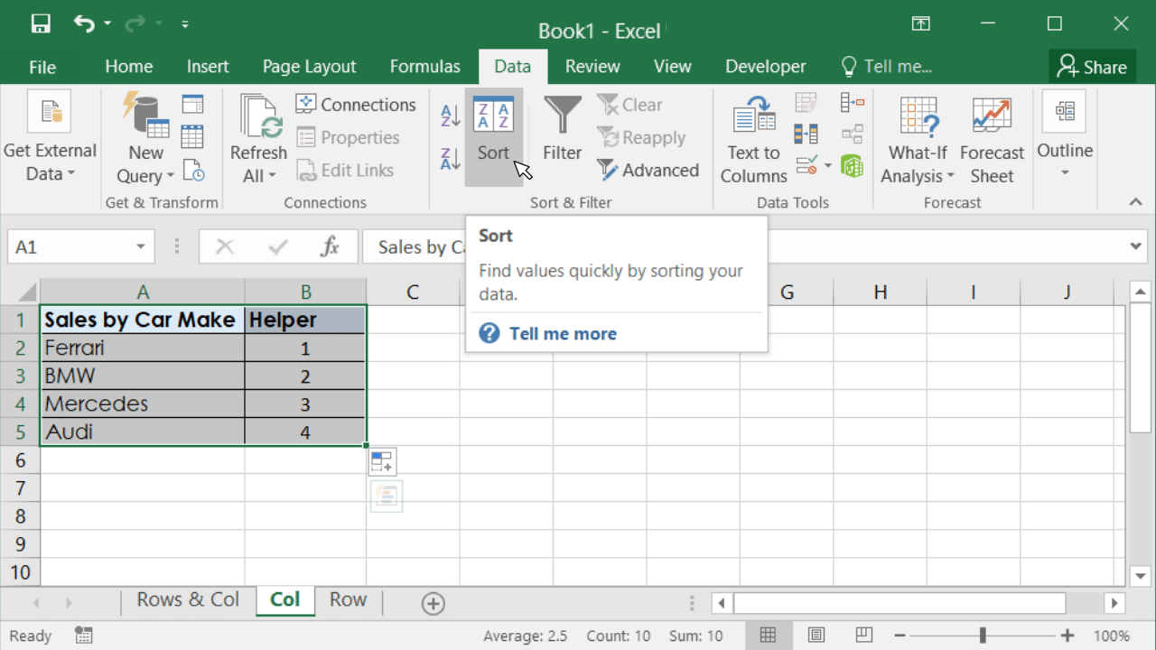
4. Click on the Sort icon to open the Sort dialog box.

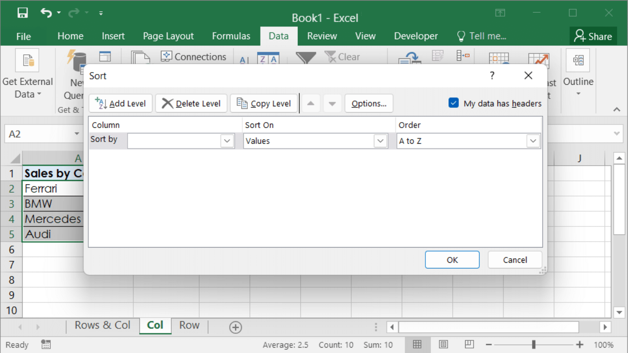
5. Select Helper from the Sort by drop down list.

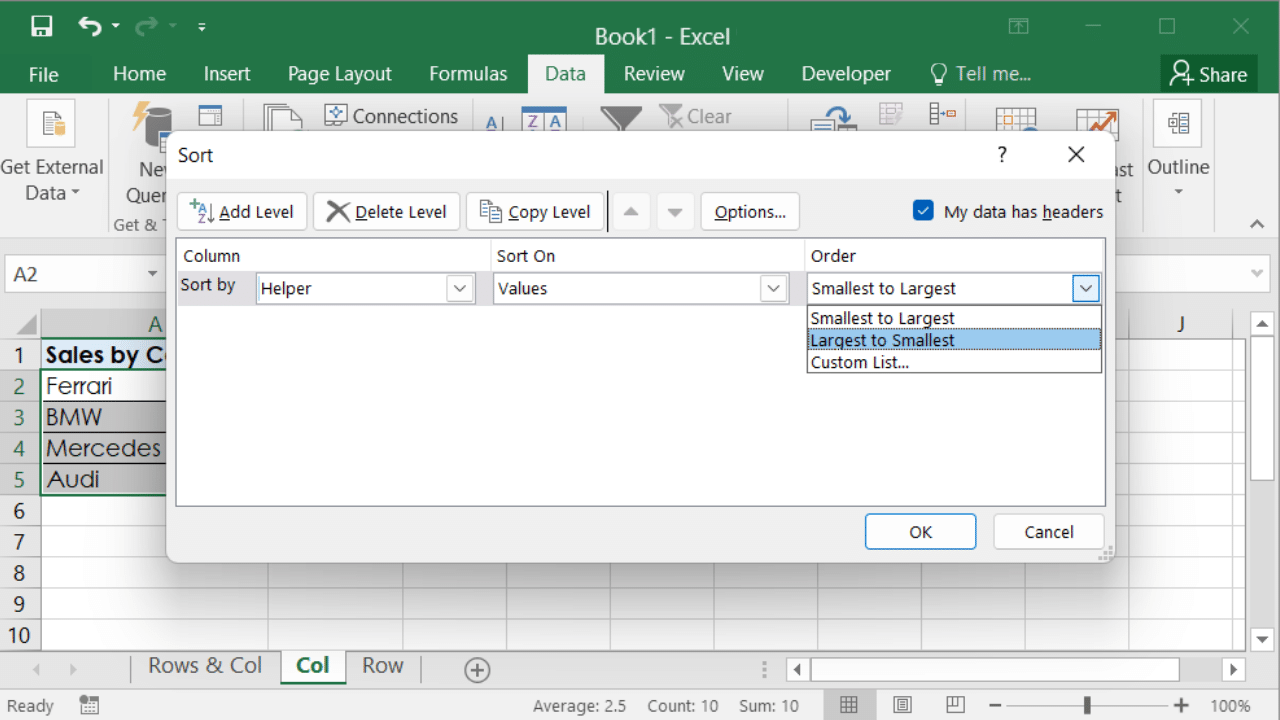
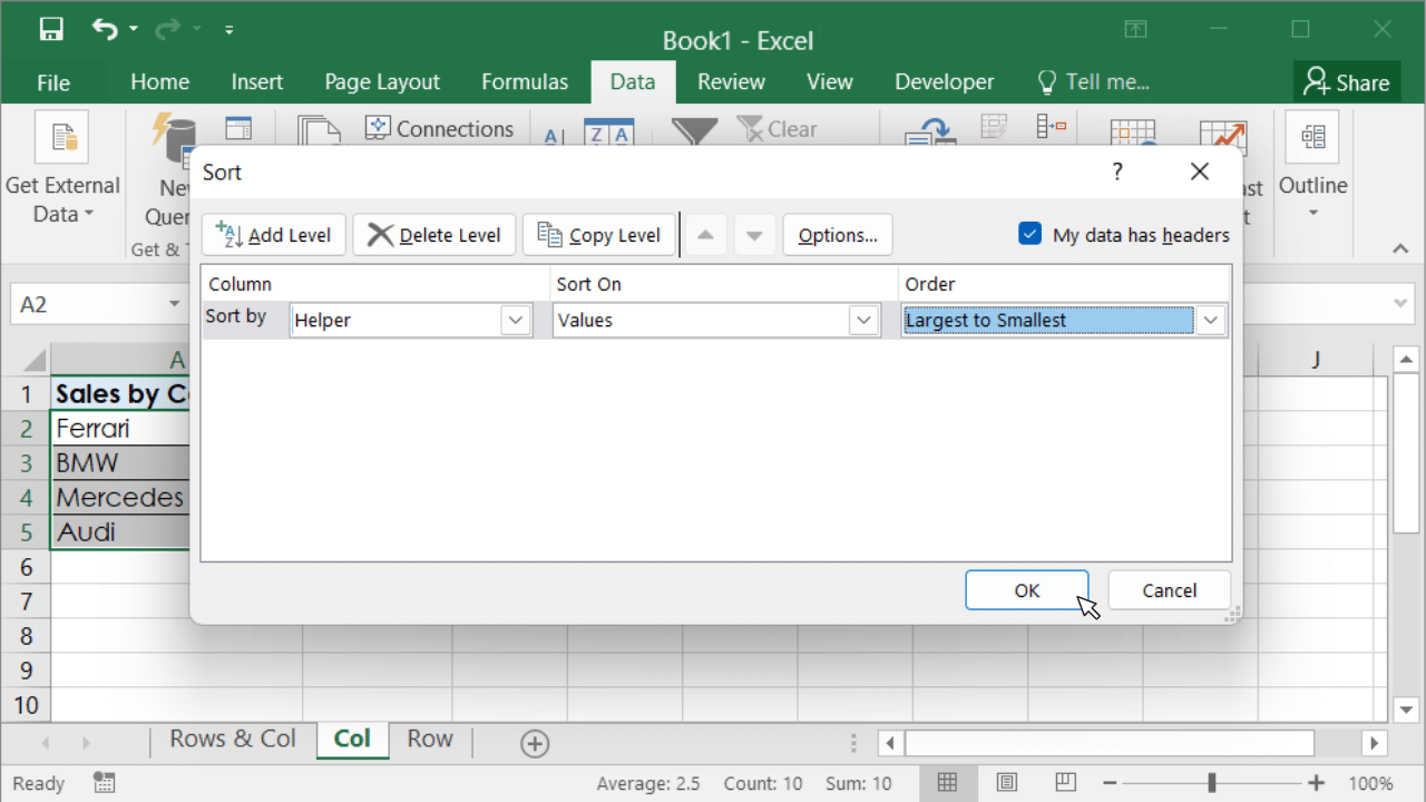
6. Select Largest to Smallest from the Order drop-down list.

7. Click OK.

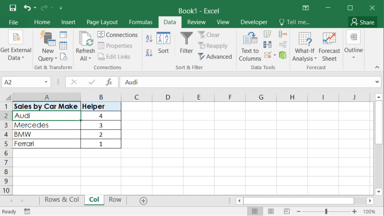
The completion of the steps above will result in the data being sorted based on the Helper column, hence, reversing the order of the data. The only purpose of the Helper column is to take on the role of a sorter column and once the data has been flipped this column can be deleted.

2.2 Using a formula

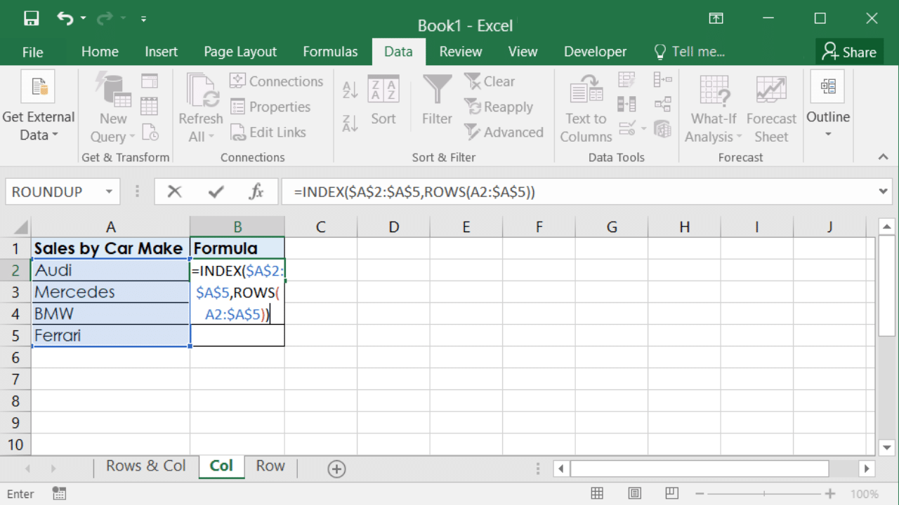
Data in a column could be flipped using a formula as well and involves fewer steps. The formula to flip data would use INDEX and ROW functions.

INDEX function returns the value of an element in a table or an array selected by the row and column number indexes.

Index Syntax INDEX(array,row_num,[column_num])

ROWS function returns the number of rows in a given range.

Rows Syntax ROWS(array)

Steps to follow:

1. To flip our sample data from the previous step, type the formula =INDEX($A$2:$A$5,ROWS(A2:$A$5)) in cell B2.

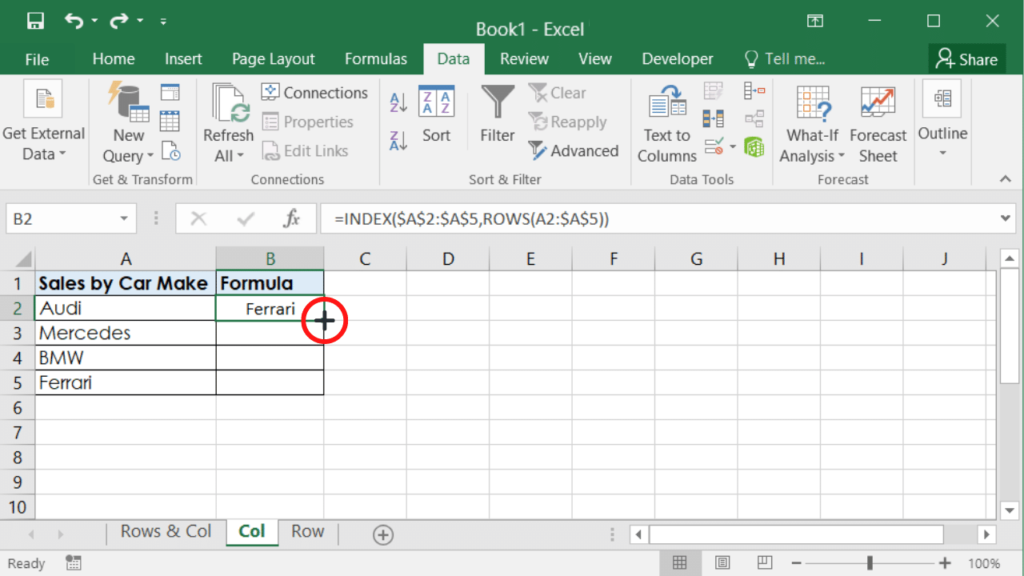
2. Copy the formula down to the rest of the cells in the column using the fill handle.

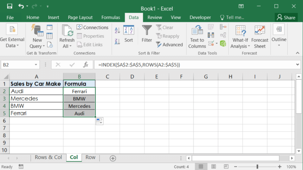
Successful completion of the above steps will result in the same list as the original column but in reverse order. This method is more useful if you are wanting to retain the original column as it is.

3. How to flip or reverse a row (using SORT and Helper row)

Using the Sort Feature to reverse data in a row could seem more challenging or impossible at first, but the method used to reverse data in a column will be the same method to be applied to reversing data in a row. This is possible due to the Sort left to right feature. This method of flipping requires an additional row Helper and the Sort Feature is then applied using the Helper row.

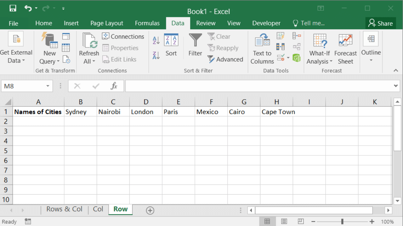
Suppose the table below is the data that is required to reverse the data in a row.

Steps to follow:

1. Enter Helper as the heading for the blank row below the row to be sorted.

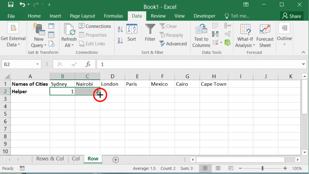
2. Enter a series of numbers start by entering 1 in the first cell, 2 in the second cell and then using the Fill handle (tip below) populate the Helper row up until the last item of the list.

Tip: Quick and easy way to number columns in MS Excel shown here

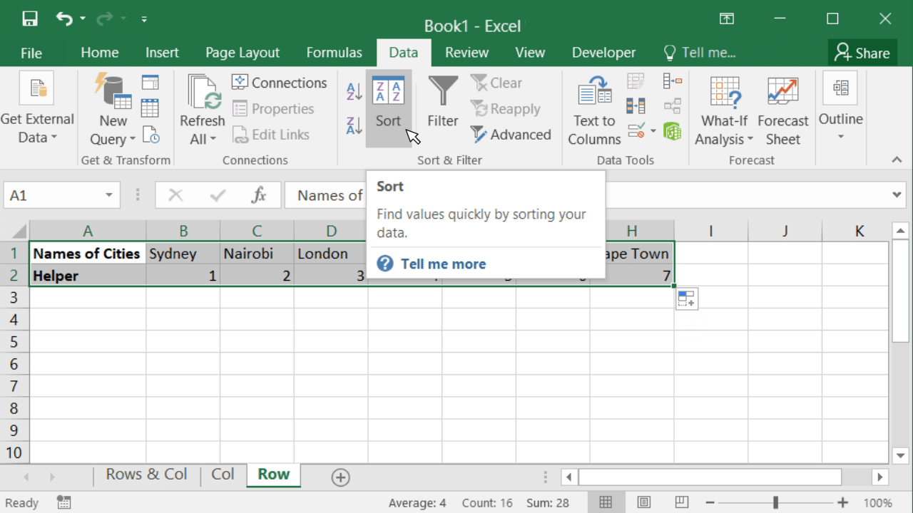
3. Select all rows with data (rows A and B in this case) and go to the Data tab. Click on the Sort icon to open the Sort dialog box.

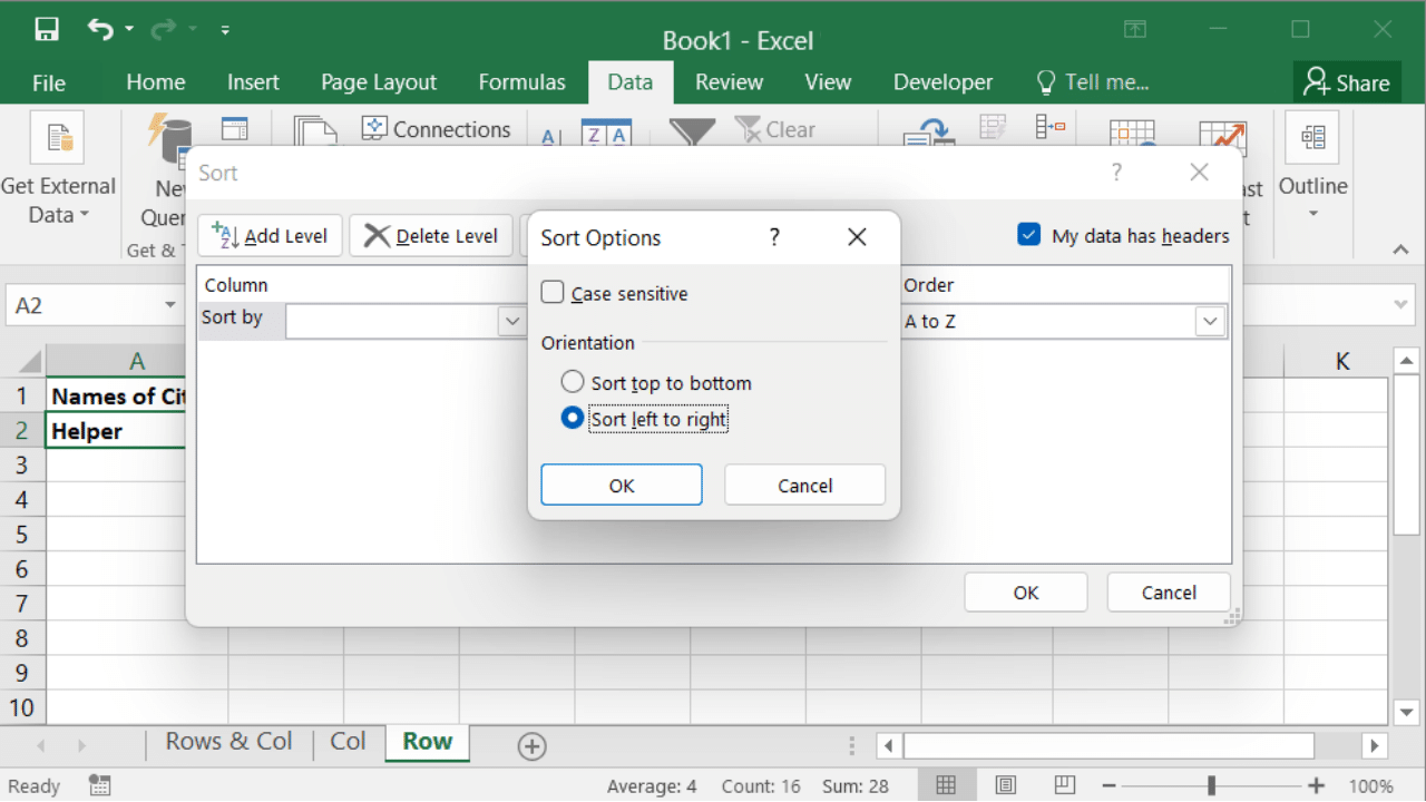
5. Click on Options.

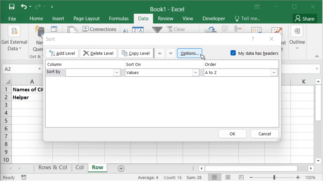
6. Select Sort left to right and click OK.

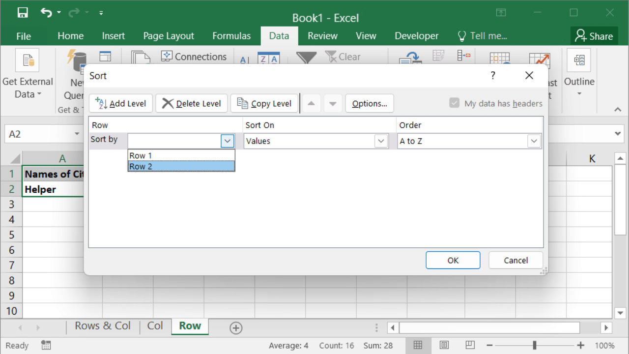
7. Choose Row 2 from the Sort by drop-down list.

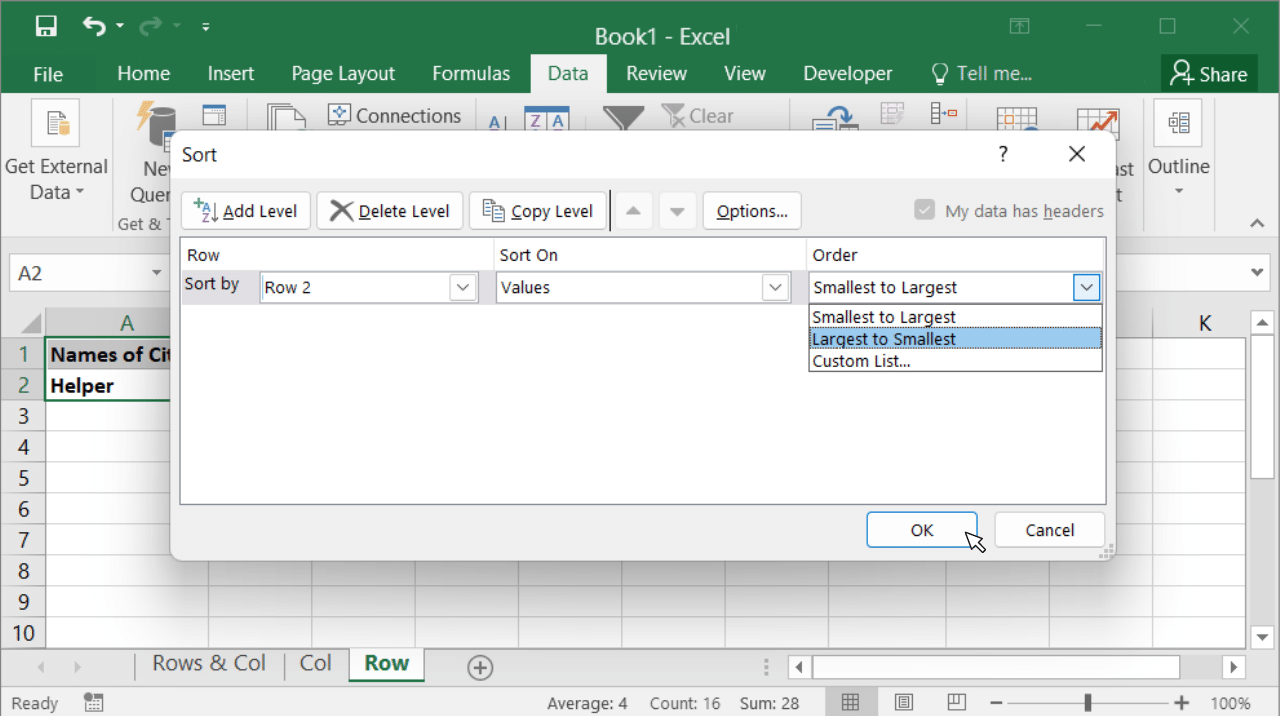
8. Select Largest to Smallest from the Order drop-down list. Click OK.

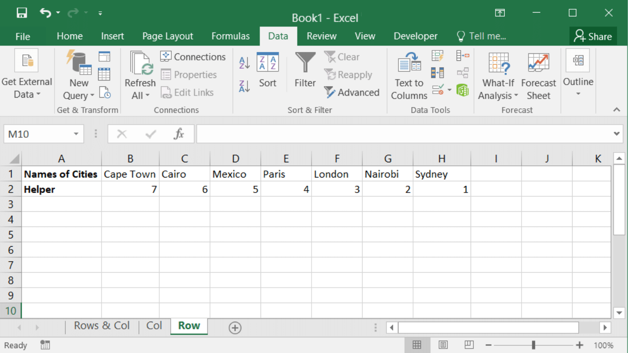
The completion of the steps above will result in the data being sorted based on the Helper row, hence, reversing the order of the data. The only purpose of the Helper row is to take on the role of a sorter row and once the data has been flipped this row can be deleted.

Quick and easy way to number rows in MS Excel

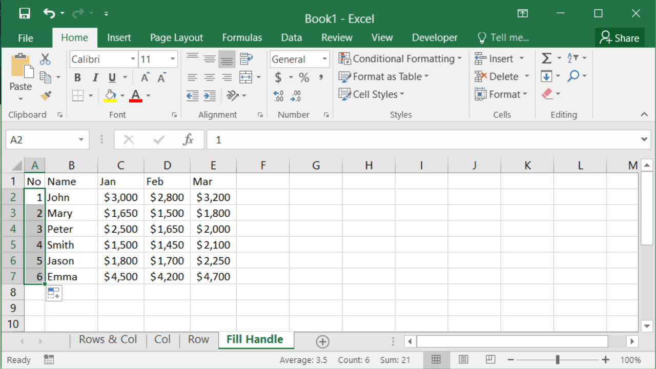
Fill handle is a function in excel that identifies a pattern in a few filled cells and it can be used to copy down the same value or a series.

Fill handle is a small square that appears in the bottom-right corner of a selected cell or range.

Hover the cursor over the small square and the cursor will change to a plus icon. You can automatically populate all the cells until the end of the dataset either by double-clicking on the plus icon or by dragging the cursor down.

Follow the steps below to copy a formula by dragging the Fill handle:

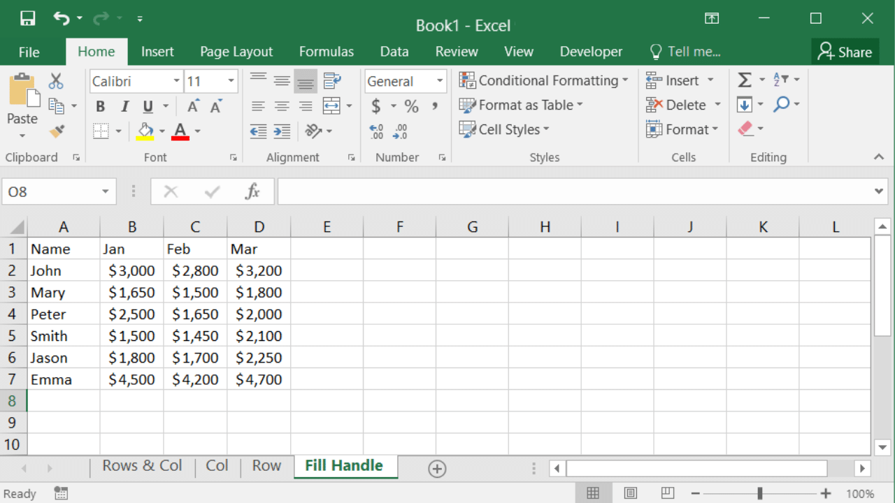
1. Suppose below is the sample data to apply Fill handle.

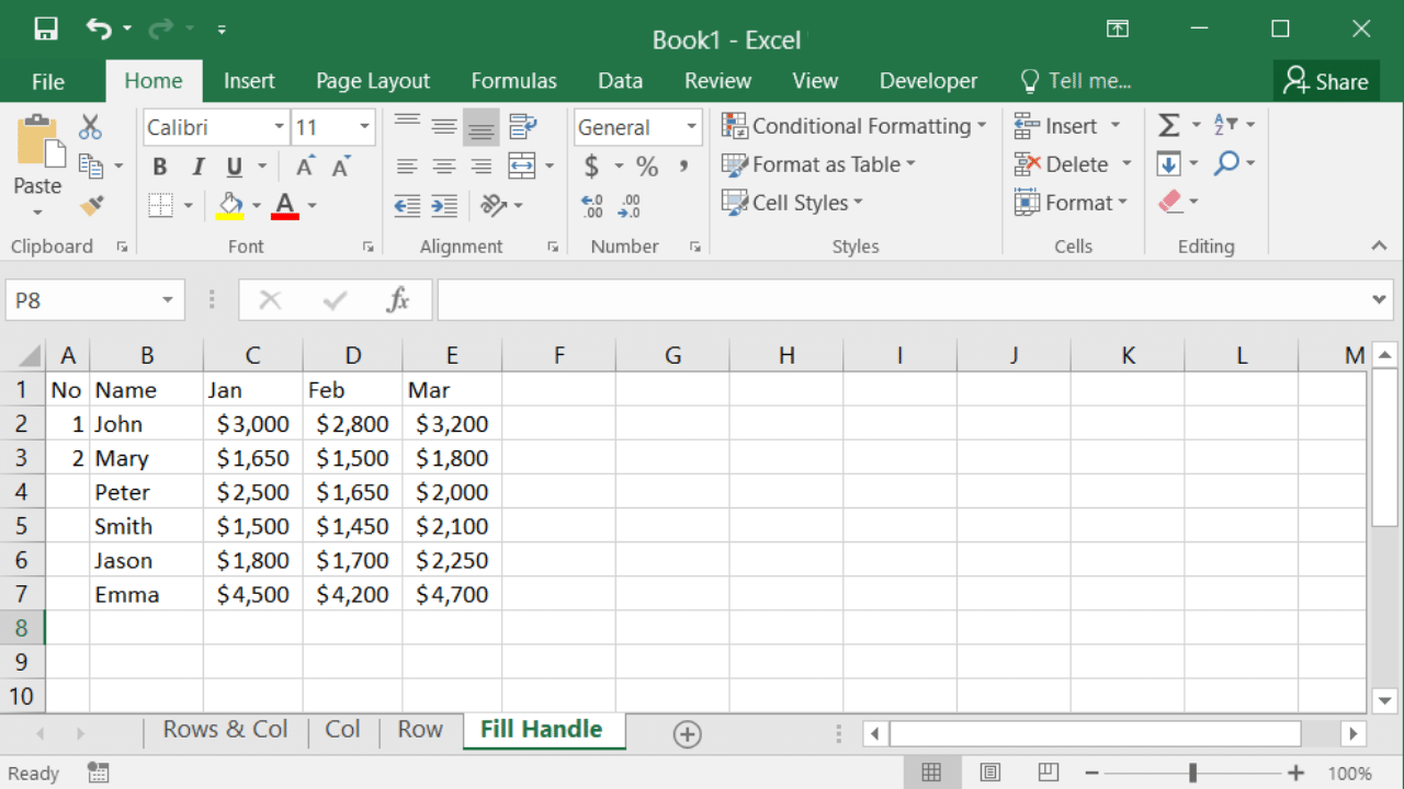
2. Enter 1 in A2, 2 in A3.

3. Select A2 and A3 and there will be a small square at the bottom right corner of the selection.

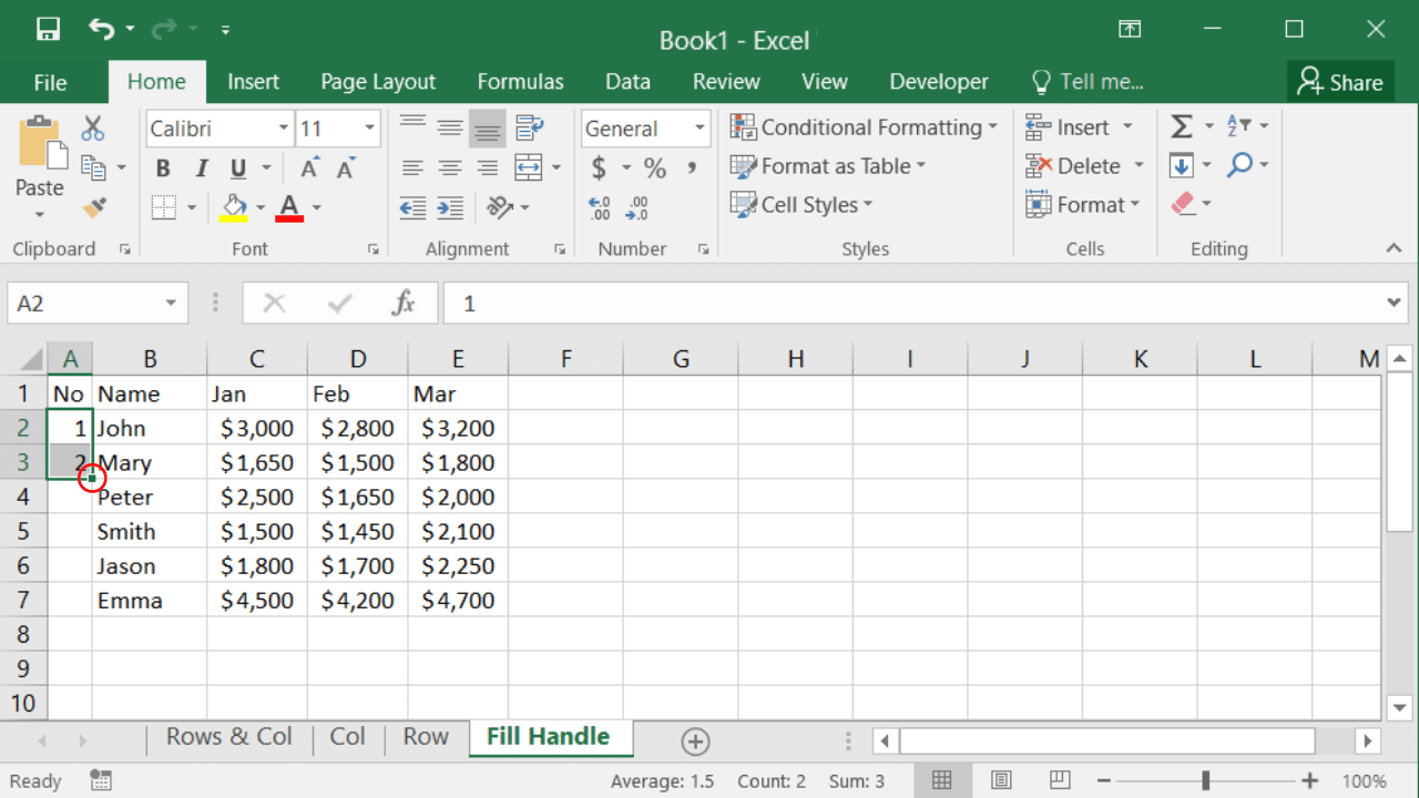
4. Hover your cursor over the small square and the cursor will change to a plus sign.

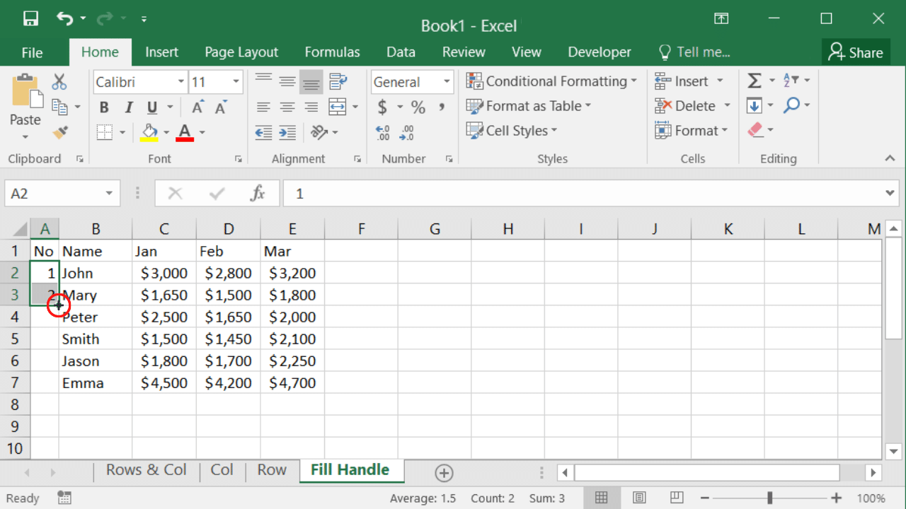
5. You can either double click on the plus sign and it will automatically fill all the cells until the end of the dataset or you could drag down the cursor until the end of the dataset.

If you have any issues with the procedure or have not been able to resolve the problem, please feel free to reach out to me using the Whatsapp button How may I help you? below or by using the comment box.